
Application of Statistics in Stormwater Management Design- a Case Study of Translating Theory into Municipal Infrastructure Development

Abstract
INTRODUCTION
Urban development replaces natural landscapes with impervious surfaces such as houses, roads, rooftops, sidewalks, parking lots, etc. These changes disrupt the natural hydrologic cycle, leading to increased surface runoff, reduced infiltration, and higher peak flows (MOE, 2003). As a result, stormwater management has become a critical component of urban infrastructure planning.
Hydrologic variables such as rainfall and runoff are inherently stochastic. Therefore, statistical methods are essential for interpreting historical datasets, predicting future conditions, and designing infrastructure systems that are both safe and cost-effective (Viessman, Lewis, & Hammer, 2009).
Below, a few statistical concepts in hydrology are presented, and thereafter a case study is presented in which a stormwater management pond has been designed, enabling sustainable urban development in the City of Hamilton, Ontario, Canada.
STATISTICAL CONCEPTS IN HYDROLOGY
Frequency Analysis and Return Period
Frequency analysis is used to estimate the probability of occurrence of rainfall events. A return period (T) represents the average recurrence interval of a storm event of given magnitude (Chow et al., 1988). For example, a 100-year storm has a 1% probability of exceedance in any given year. Normally used design storms in urban stormwater management system design are 2-year, 5-year, 25-year, and 100-year events.
Regression Analysis, Coefficient of Determination (R²), Nash–Sutcliffe Efficiency (NSE)
Regression Analysis
Regression analysis is a core statistical method used to develop empirical relationships between hydrologic variables. Hydrologic systems are influenced by multiple interacting factors including rainfall intensity, watershed area, slope, soil type, and land use. Regression techniques allow these relationships to be quantified mathematically for prediction and design purposes (Chow et al., 1988).
In stormwater engineering, regression is commonly used to estimate peak discharge, runoff volume, and runoff coefficients based on rainfall and watershed characteristics. A simple linear regression model is expressed as:
Y = a + bX; where Y represents the dependent variable (i.e., peak flow), X represents the independent variable (i.e. the water level).
Coefficient of Determination (R2)
The coefficient of determination (R2) is one of the most commonly used statistical indicators for evaluating the performance of regression models and hydrologic simulations. It measures the proportion of variance in the observed dataset that is explained by the predictive model. In hydrologic applications, (R2) provides an indication of how well simulated values reproduce the variability observed in measured data (Moriasi et al., 2007).
Values of R2 range from 0 to 1, where a value of 1 indicates perfect agreement between observed and predicted values, while a value close to 0 indicates little or no correlation. During hydrologic model calibration, engineers often seek to maximize (R2) to improve confidence in model predictions and ensure that the model adequately captures watershed response characteristics.
Although high R2 values generally indicate good model performance, researchers have noted that R2 alone may not fully represent predictive accuracy because it primarily measures correlation rather than the magnitude of prediction errors (Legates & McCabe, 1999). Consequently, R2 is often used in conjunction with other performance indicators such as the Nash–Sutcliffe Efficiency (NSE) to provide a more comprehensive evaluation of hydrologic model performance.
Nash–Sutcliffe Efficiency (NSE)
The Nash–Sutcliffe Efficiency (NSE), originally developed by Nash and Sutcliffe (1970), is one of the most widely accepted performance measures for hydrologic model calibration and validation. Unlike the coefficient of determination, which primarily measures correlation, NSE evaluates how closely simulated values match observed values by comparing the residual variance of the model predictions with the variance of the observed data. The NSE is expressed as:
; where Model predicted value at time t; = Observed value at time t; =Mean of the observed data over the entire evaluation period; T= Total number of time steps
In stormwater management applications, NSE is frequently used during model calibration to evaluate simulated hydrographs, runoff volumes, and peak discharge estimates. Because NSE directly accounts for prediction errors, it is often regarded as one of the most robust and informative performance indicators for assessing the reliability of hydrologic and hydraulic models used in stormwater infrastructure design.
Intensity-Duration-Frequency (IDF) Curves
IDF curves define rainfall intensity as a function of storm duration and return period. For a particular return period, the average intensity (I) of rainfall of duration T can be calculated based on the following equation:
; where a, b, and c are IDF coefficients that are unique to each municipality. IDF coefficients are developed for each municipality by analyzing long-term (i.e. 30 years) rainfall records of different durations and frequencies.
Rating Curves and Application of Regression
A rating curve defines the relationship between water level (stage) and discharge in open channels or hydraulic structures. Because continuous flow measurement is difficult, stage is measured and converted to discharge using empirical relationships derived from regression analysis (ASCE, 1996). The general form of a rating curve is:
; where Q is discharge, H is water level, H₀ is zero-flow stage, and a and b are regression coefficients.
Rating curves are widely used in: Stormwater Pond outlet calibration, River discharge estimation, Flood forecasting, Hydrologic model validation, etc. In stormwater management ponds, rating curves define outlet structure performance, ensuring that controlled release rates meet municipal criteria under varying water levels.
CASE STUDY: STORMWATER MANAGEMENT POND DESIGN
Project Overview
The study area is located (in the City of Hamilton) south of Rymal Road East and West of Highway 56 (HWY56); previously greenfield (undeveloped land) has been proposed to be developed as a subdivision. The subject site is about 71.33 ha. In pre-development conditions, this vast undeveloped land drains through localized channels that pass through the existing culvert under Swayze Road, connecting to the local ditches through the existing subdivision east of Swayze Road, ultimately draining to Sinkhole Creek (A tributary of Twenty Mile Creek located south of HWY56).
Obviously, the proposed subdivision development will increase the impervious cover at the subject site which will increase runoff and uncontrolled runoff from the proposed development will overburden the downstream reaches of Sinkhole Creek. Furthermore, a ‘Rapid Geomorphic Assessment’ (RGA) study identified that some reaches of Sinkhole Creek are vulnerable to erosion under existing conditions.
Therefore, as one of the requirements of the approval for the proposed subdivision development at the subject site, the local municipality (The City of Hamilton) demanded that the runoff release rate for 2 to100 year storm events from the subject development should not exceed the corresponding predevelopment level and the predevelopment level 2- to 100-year flow target at Sinkhole Creek should be determined based on existing conditions model calibration.
Methodology
In order to meet the City requirements for the stormwater management approval, the following methodology was adopted in the analysis and design:
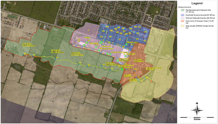
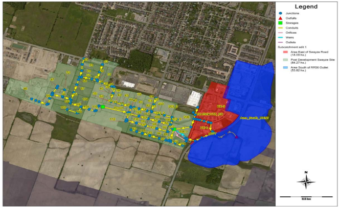
Step 1: The existing conditions hydrologic model was created. PCSWMM model was selected for hydrologic and hydraulic modeling for this project. The subject development site is 71.33 ha; in addition to that there is an existing subdivision to the north known as Deerfield Estate (which has its own stormwater management pond providing stormwater runoff quantity and quality control), 26.49 commercial lands known as Walmart lands (which also has its own stormwater management pond providing stormwater quantity and quality control for this area) both outlets to the road side ditches along Swayze road which being conveyed through the Swayze culvert and ultimately outlets to the Sinkhole Creek through exiting culvert at HWY56. In addition, drainage analysis reveals that there is an additional 71.91 ha area that drains to the Sinkhole Creek storm outlet under existing conditions. The existing conditions model was built (PCSWMM model) and is presented in Figure 1. Figure 2 shows the proposed conditions of the PCSWMM Model at the subject site.
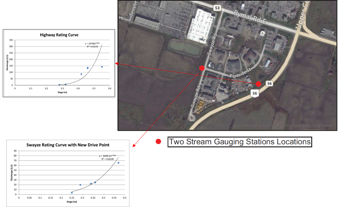
Step 2: Rainfall data were obtained from gauging stations, and corresponding water levels were obtained from flow monitoring locations. Water level data were then converted to discharge data by using the rating curve or equation developed for the gauging stations. The flow monitoring locations or gauging stations and corresponding rating curves/equations can be found in Figure 3.
|
|
|
|---|---|
|
Figure 1: Existing Conditions PCSWMM Model of the Study Area |
Figure 2: Proposed Conditions PCSWMM Model of the Subject Site |
|
|
|
|
Figure 3: Flow Monitoring Location and Corresponding Rating Curve/ Equation |
|
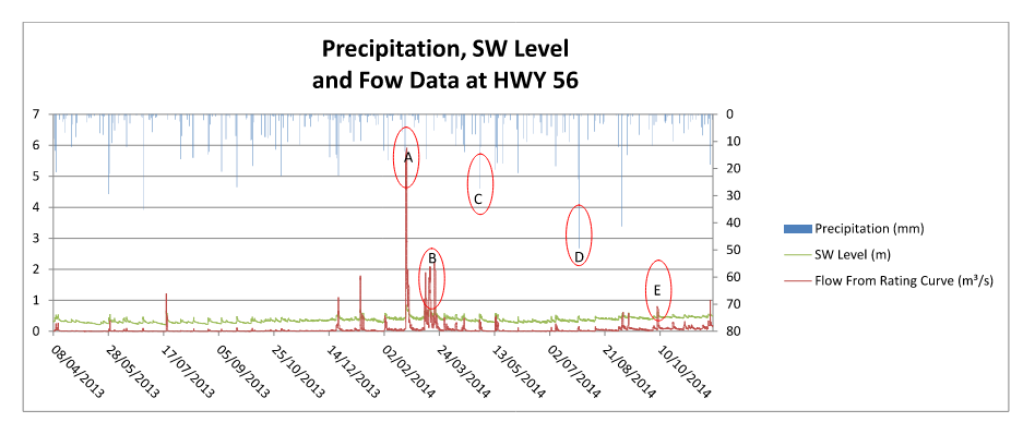
The observed rainfall and corresponding discharge data were available from 08 April 2013 to 26 November 2014. The data were then scanned, and outlier values were discarded from analyses. Outlier values are high discharge or water level value but corresponding low rainfall inputs and vice versa. The observed rainfall data and corresponding flow data (for the duration of 08 April 2013 to 26 November 2014) can be seen in Figure 4 and some of the outlier values are circled on this figure as example. Rainfall events less than 2.5 mm were discarded from the analyses.
Finally, two sets of the observed rainfall and discharge data were selected: one set (from April 25 to August 21, 2013) was used for model calibration, and another set (from April 01 to August 31, 2014) has been used in model validation. The duration for calibration and validation (from April to August of two different years) selected such that hydrologic response in terms of flow is high due to spring melt and rainfall inputs at this time of the year in Hamilton region. The understanding was that studying the hydrologic response during high flow season would provide good confidence in the model calibration results.
|
|
|---|
|
Figure 4: Observed Rainfall, Corresponding Water Level and Flow Data |
Step 3: Based on the observed flow data (obtained in step 2 above), the existing conditions model was calibrated based on the statistical analysis. With the selected observed rainfall and discharge data the model hydrological parameters such as sub-catchment width, CN values, depression storage, etc. were adjusted (i.e. Calibrated) such that there is acceptable model flow prediction based on the observed discharge value. The statistical parameters R² >0.5 and NSE>0 was considered to be the minimum acceptable limit of the correlation between the model computed and observed values.
Step 4: Sensitivity analysis was performed with 2 to 100 year design storm events of various durations (3 hour, 6 hour,12 hourr, 24 hour) and type (SCS, Chicago). Based on the sensitivity analysis results, Chicago 24 hour rainfall (2 year to 100 year return period) was selected as the design rainfall. The 24 hour design rainfall depth for different frequency or return periods (2 to 100 year) was determined based on City of Hamilton’s IDF curves.
Step 5: The existing condition hydrologic was run with design storm events with 2 year, 5 year, 10 year, 25 year, 50 year and 100 year return periods to set the predevelopment target release rate which should be maintained in the post development conditions for the respective storm events. Then the target predevelopment flow for 2 to 100 year storm events were found my running the existing conditions calibrated model with corresponding design storm events (Chicago 24 hour).
Step 6: In the next step, post development hydrologic and hydraulic model (using proposed subdivision land use such as roads, houses, stormwater management pond etc.) was created in PCSWMM model. The subdivision development proposed two stormwater management pond. One dry pond for providing stormwater quantity control for upstream lands and one wet pond providing further stormwater quantity control as well as quality control for all upstream lands including the subject site (71.33 ha), Deerfield and Walmart site. The post development was created in PCSWM model with the aid of GIS software such as AutoCAD Civil 3D and free domain GIS platform such as SAGA GIS to transform the CAD data into Esri Shape file format for import in the model. The post development PCSWMM model can be seen in Figure 2. The released flow from Deerfield and Walmart site has been added as an inflow to the hydraulic node, for this reason, the sub-catchment representation of these two sites are not shown on the post development PCSWMM model.
Step 7: With calibrated model parameters (obtained in Step 3 above), the post development model was then run with the design rainfall with various return period (i.e. 2 year, 5 year, 10 year, 50 year and 100 year) and SWM pond was designed (i.e. flow control orifice and weir were sized) so that the released discharge at the Sinkhole Creek Outlet does not exceed the predevelopment flow target obtained Step 4). Regression-based rating curves were used to define outlet discharge characteristics of the stormwater management pond.
|
|
|
|---|---|
|
(a) |
(b) |
|
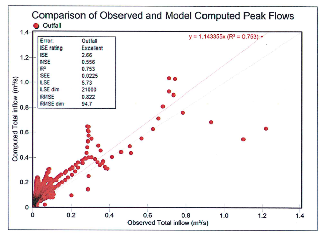
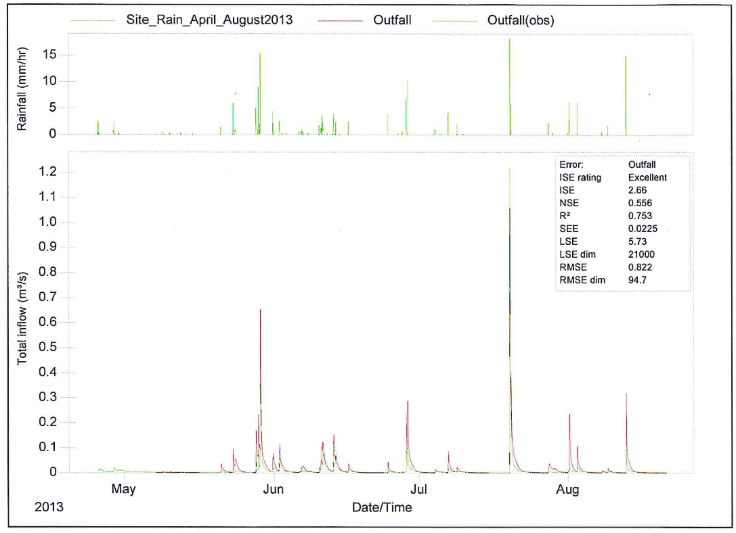
Figure 5: a) Calibration Model Run from April 25 to August 21, 2013. (R² = 0.753 and Slope of the Line of Regression = 1.14); b) shows observed and model-computed hydrograph during calibration model run |
|
|
|
|
|---|---|
|
(a) |
(b) |
|
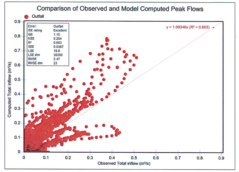
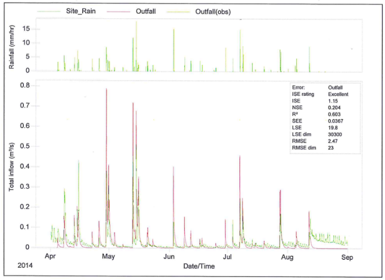
Figure 6: a) Validation Model Run from April 01 to August 31, 2014; (R² = 0.603 and Slope of the Line of Regression = 1.00); b) shows observed and model computed hydrograph for the validation model run |
|
RESULTS AND DISCUSSIONS
Figure 5 shows the R² =0.7 and NSE= 0.556 for the calibration model run in PCSWMM with observed rainfall and discharge data (from April 25 to Augst 21, 2013). The slope of the Regression line between model predicted and observed flow is 1.14 (close to 1), which suggests good correlation between the model predicted and observed values.
With the same calibrated parameters, the existing conditions PCSWMM model was re-run with the second set of observed rainfall and flow data (for the period of April 01 to August 31, 2014) for model validation (i.e. to further validate the performance of model prediction). Figure 6 shows R² =0.603 and NSE= 0.204 for the validation model run (from April 01 to Augst 31, 2014). The slope of the regression line is also almost 1 which indicates very good correlation between the observed and predicted flow and very good confidence in the model predictability (i.e. model calibration).
Based on the above, the statistical parameter values helped to decide on the confidence level of the model calibration, and based on the calibrated model, the SWM pond was designed and further refined based on the advice from the municipality and a peer review consultant before obtaining final approval from the approval authorities – City of Hamilton.
CONCLUSIONS
Statistical concepts are essential in hydrology and stormwater management design. Methods such as frequency analysis, regression modeling, and rating curve development provide the foundation for modern engineering practice. The case study demonstrates that integrating statistical tools into stormwater pond design enables effective flood control, regulatory compliance, and sustainable urban development.
REFERENCES
ASCE.1996. Hydrology handbook (2nd ed.). American Society of Civil Engineers.
Chow, V. T., Maidment, D. R., & Mays, L. W.1988. Applied hydrology. McGraw-Hill.
Legates, D. R., & McCabe, G. J.1999. Evaluating the use of "goodness-of-fit" measures in hydrologic and hydroclimatic model validation. Water Resources Research, 35(1), 233–241.
Moriasi, D. N., Arnold, J. G., Van Liew, M. W., Bingner, R. L., Harmel, R. D., & Veith, T. L.2007. Model evaluation guidelines for systematic quantification of accuracy in watershed simulations. Transactions of the ASABE, 50(3), 885–900.
Nash, J. E., & Sutcliffe, J. V. 1970. River flow forecasting through conceptual models part I—A discussion of principles. Journal of Hydrology, 10(3), 282–290.
Ontario Ministry of the Environment (MOE). 2003. Stormwater management planning and design manual.
Viessman, W., Lewis, G. L., & Hammer, M. J. 2009. Introduction to hydrology. Pearson Education.
Acknowledgement: The author acknowledges sincere thanks to all staff at A.J. Clarke and Associates Ltd. for their sincere support and help in carrying out the study (in 2016); especially, Adi Irani, P.Eng.; Claudio Giammarco, P.Eng.; Bozena Bednarska, P.Eng.

Comments 0
No comments yet. Be the first to comment!
Sign in to leave a comment.